Simulation of Synthetic Cells (AnnData Object)#
Building OneSC simulator#
After the inference of GRNs from previous step, we can perform simulations using the GRN as a backbone. You can download the inferred GRN from previous step here. For all simulations, we need to define the initial state. In our case, we know that cells start in the CMP state. To determine the Boolean state of genes in the CMP state, we subset the adata to those cells and then apply thresholds on the mean expression and the percent of cells in which the gene is detected:
boolean_states_df = onesc.define_boolean_states_anndata(adata, cluster_col = 'cell_types')
xstates = boolean_states_df['CMP'] * 2
Now we construct a OneSC simulator object:
netname = 'CMPdiff'
netsim = onesc.network_structure()
netsim.fit_grn(iGRN)
sim = onesc.OneSC_simulator()
sim.add_network_compilation(netname, netsim)
Simulate wildtype trajectory#
Finally we are ready to simulate expression state trajectories using our GRN.
OneSC_simulator: the OneSC simulator object to use.
initial_exp_dict (dict): dictionary of initial state values.
network_name (str): the name of the fitted gene regulatory network structure that the user want to use for simulation.
perturb_dict (dict, optional): a dictionary with the key of gene name and value indicating the in silico perturbation. If the user want to perform overexpression, then set the value between 0 and 2. If the user want to perform knockdown, then set the value between 0 and -2. Defaults to dict().
num_runs (int, optional): number of simulations to run. Defaults to 10.
n_cores (int, optional): number of cores for parallel computing. Defaults to 2.
num_sim (int, optional): number of simulation steps. Defaults to 1000.
t_interval (float, optional): the size of the simulation step. Defaults to 0.01.
noise_amp (int, optional): the amplitude of noise. Defaults to 0.1
simlist_wt = onesc.simulate_parallel_adata(sim, xstates, netname, n_cores = 8, num_sim = 1000, num_runs = 32, t_interval = 0.1, noise_amp = 0.5)
simulate_parallel_adata returns a list of annData objects. Each annData contains num_sim simulated cells starting at the initial_exp_dict state, and progressing subject to the regulatory constraints defined by the provided GRN modulated by randomly generated noise (if allowed). Each annData has .obs[‘sim_time’].
Setup PySCN for classification#
We will use PySCN to annotate the states of the simulated cells. Train the classifer now:
adTrain_rank, adHeldOut_rank = pySCN.splitCommonAnnData(adata, ncells=50,dLevel="cell_types")
clf = pySCN.train_rank_classifier(adTrain_rank, dLevel="cell_types")
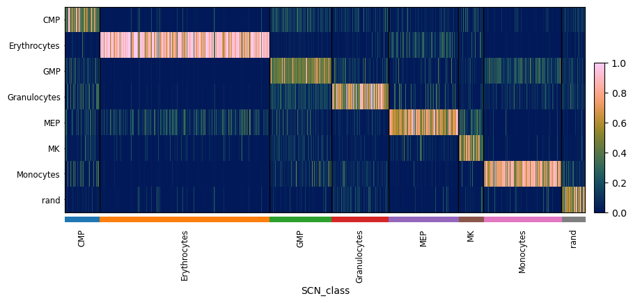
Classify held out data:
pySCN.rank_classify(adHeldOut_rank, clf)
pySCN.heatmap_scores(adHeldOut_rank, groupby='SCN_class')
 Note: the function
 train_rank_classifier() ranks transforms training and query data instead of TSP. Be forewarned that it is likely to be slow if applied to adata objects with a lot of genes.
Classify Simulated Cells#
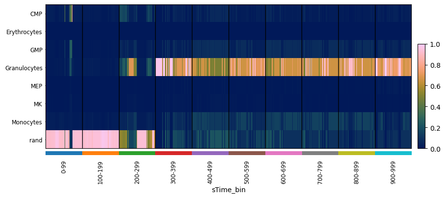
Let’s look at the transcriptomic states over sim_time for one simulated trajectory. We will classify the cells first, and then visualize
ad_sim1 = simlist_wt[0].copy()
pySCN.rank_classify(ad_sim1, clf)

# a hack because sc.pl.heatmap requires a 'groupby', so groupby simulation time bin
tmp_obs = ad_sim1.obs.copy()
bins = np.linspace(-1, 999, 11)
labels = [f"{int(bins[i]) + 1}-{int(bins[i+1])}" for i in range(len(bins)-1)]

tmp_obs['sTime_bin'] = pd.cut(tmp_obs['sim_time'], bins=bins, labels=labels)
ad_sim1.obs = tmp_obs

pySCN.heatmap_scores(ad_sim1, groupby = 'sTime_bin')
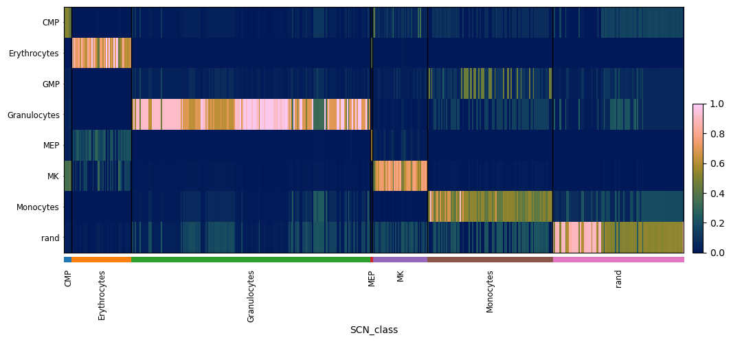
 Instead of looking the trajectory of a single cell, we can sample the end stages of all simulations:
ad_wt = onesc.sample_and_compile_anndatas(simlist_wt, X=50, time_bin=(80, 100), sequential_order_column='sim_time')
pySCN.rank_classify(ad_wt, clf)
pySCN.heatmap_scores(ad_wt, groupby = 'SCN_class')
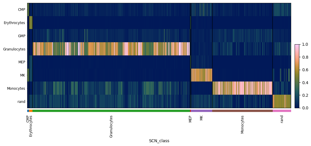
Simulate knockout trajectory#
Now, let’s simulate trajectories of cells in which Cebpa is knocked out
perturb_dict = dict()
perturb_dict['Cebpa'] = -1
simlist_cebpa_ko = onesc.simulate_parallel_adata(sim, xstates, 'CMPdiff', perturb_dict = perturb_dict, n_cores = 8, num_sim = 1000, t_interval = 0.1, noise_amp = 0.5)
Now fetch the simulated cells, sampling from the end stages, classify them, and visualize the results.
ad_cebpa_ko = onesc.sample_and_compile_anndatas(simlist_cebpa_ko, X=50, time_bin=(80, 100), sequential_order_column='sim_time')
pySCN.rank_classify(ad_cebpa_ko, clf)
pySCN.heatmap_scores(ad_cebpa_ko, groupby = 'SCN_class')
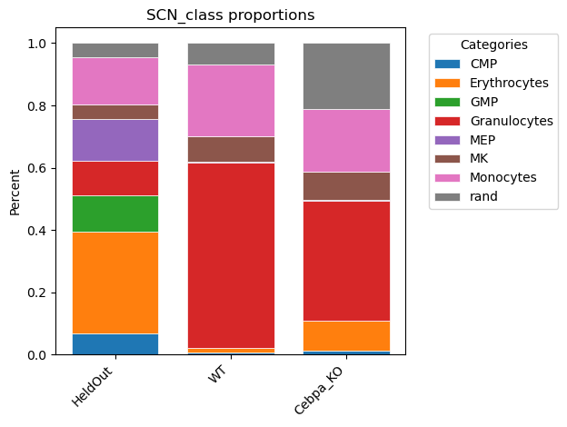
 We can also directly compare the proportions of cell types across simulations/perturbations as follows:
pySCN.plot_cell_type_proportions([adHeldOut_rank,ad_wt, ad_cebpa_ko], obs_column = "SCN_class", labels=["HeldOut", "WT","Cebpa_KO"])
If we want to perform multiple perturbations, we can add that into the perturb dict, and pass that into the simulation function.
perturb_dict = dict()
perturb_dict['Cepbe'] = -1
perturb_dict['Gata2] = 1